
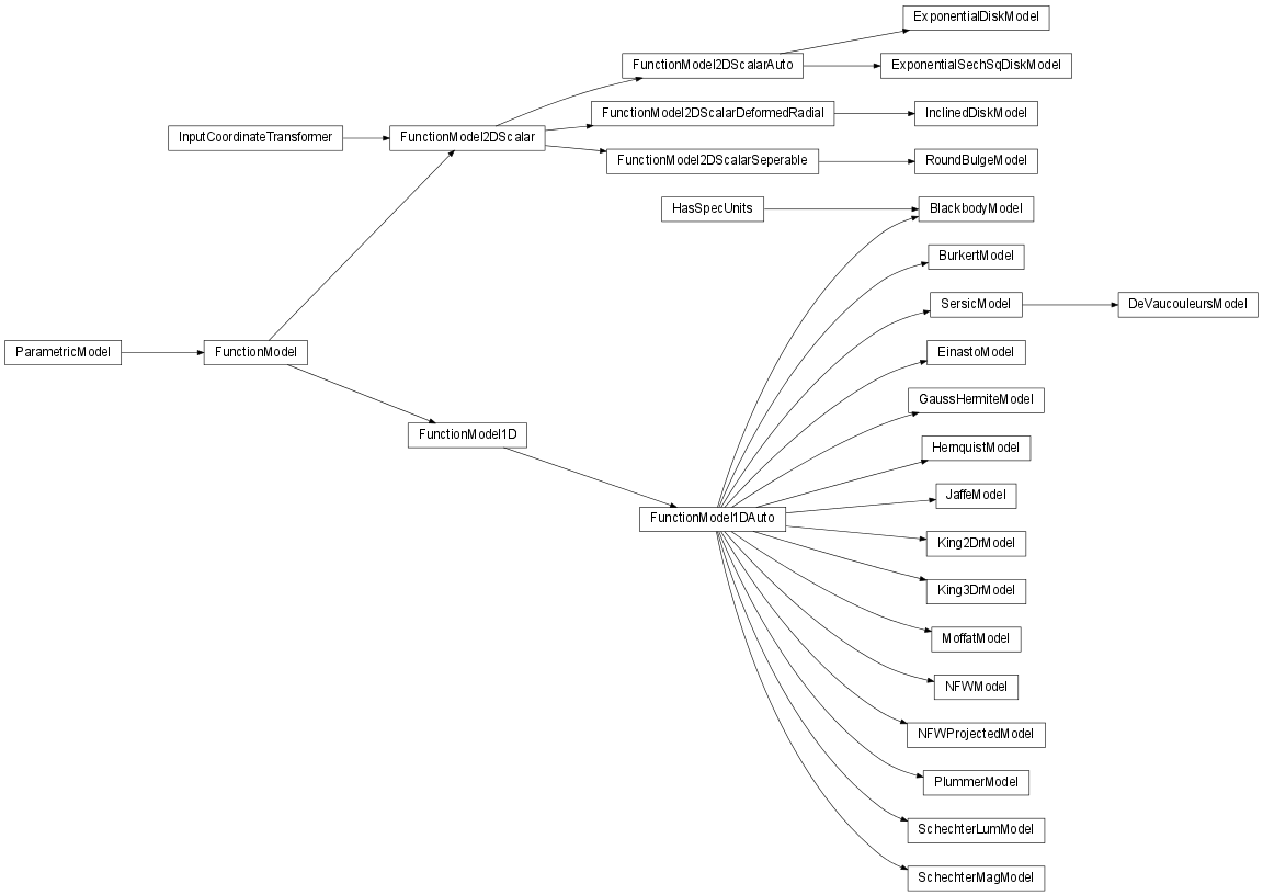
This module makes use of the pymodelfit package to define a number of models inteded for data-fitting that are astronomy-specific. Note that pymodelfit was originally written as part of astropysics, and hence it is tightly integrated (including the Fit GUI, where relevant) to other parts of astropysics, often using the models in this module.
Note
Everything in the pymodelfit package is imported to this package. This is rather bad form, but is currently done because other parts of astropysics is written for when pymodelfit was part of astropysics. This may change in the future, though, so it is recommended that user code always use from pymodelfit import ... instead of from astropysics.models import ....
Bases: pymodelfit.core.FunctionModel1DAuto, astropysics.spec.HasSpecUnits
A Planck blackbody radiation model.
Output/y-axis is taken to to be specific intensity.
Returns the flux density at the requested wavelength for a blackbody of the given radius at a specified distance.
| Parameters: | |
|---|---|
| Returns: | flux/wl at the specified distance from the blackbody |
Determines the distance to a spherical blackbody of the specified radius assuming the flux is given by the model at the given temperature.
Determines the radius of a spherical blackbody at the specified distance assuming the flux is given by the model at the given temperature.
Sets A so that the output is the flux at the specified distance from a spherical blackbody with the specified radius.
| Parameters: |
|---|
Sets A so that the output is specific intensity/surface brightness.
assumes cgs units
Uses the Wien Displacement Law to calculate the temperature given a peak input location (wavelength, frequency, etc) or compute the peak location given the current temperature.
| Parameters: | peakval (float or None) – The peak value of the model to use to compute the new temperature. |
|---|---|
| Returns: | The temperature for the provided peak location or the peak location for the current temperature if peakval is None. |
Bases: pymodelfit.core.FunctionModel1DAuto
Burkert (1996) profile defined as:
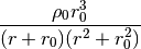
where rho0 is the central density.
Bases: astropysics.models.SersicModel
Sersic model with n=4.
Bases: pymodelfit.core.FunctionModel1DAuto
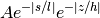
Einasto profile given by

A is the density where the log-slope is -2, and rs is the corresponding radius. The alpha parameter defaults to .17 as suggested by Navarro et al. 2010
Note
The Einasto profile is is mathematically identical to the Sersic profile (SersicModel), although the parameterization is different. By Convention, Sersic generally refers to a 2D surface brightness/surface density profile, while Einasto is usually treated as a 3D density profile.
Bases: pymodelfit.core.FunctionModel2DScalarAuto
A disk with an exponential profile along both vertical and horizontal axes. The first coordinate is the horizontal/in-disk coordinate (scaled by l) wile the second is z. i.e.
for pa = 0 ; non-0 pa rotates the profile counter-clockwise by pa radians.
Bases: pymodelfit.core.FunctionModel2DScalarAuto
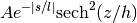
A disk that is exponential along the horizontal/in-disk (first) coordinate,
and follows a  profile along the vertical (second)
coordinate. i.e.
profile along the vertical (second)
coordinate. i.e.
for pa = 0 ; non-0 pa rotates the profile counter-clockwise by pa radians.
Bases: pymodelfit.core.FunctionModel1DAuto
Model notation adapted from van der Marel et al 94
hj3 are h3,h4,h5,... (e.g. N=len(hj3)+2 )
compute the requested moment on the supplied function, or this object if f is None
Bases: pymodelfit.core.FunctionModel1DAuto
Hernquist (1990) profile defined as:

where A is the total mass enclosed. Note that r0 does not
enclose half the mass - the radius enclosing half the mass is
 .
.
Note
This form is equivalent to an AlphaBetaGammaModel with
 , but with a slightly
different overall normalization.
, but with a slightly
different overall normalization.
Bases: pymodelfit.core.FunctionModel2DScalarDeformedRadial
Inclined Disk model – identical to FunctionModel2DScalarDeformedRadial but with inclination (inc and incdeg) and position angle (pa and padeg) in place of axis-ratios.
Bases: pymodelfit.core.FunctionModel1DAuto
Jaffe (1983) profile as defined in Binney & Tremaine as:
where A is the total mass enclosed. rj is the radius that encloses half the mass.
Note
This form is equivalent to an AlphaBetaGammaModel with
 , but with a slightly
different overall normalization.
, but with a slightly
different overall normalization.
Bases: pymodelfit.core.FunctionModel1DAuto
2D (projected/surface brightness) King model of the form:
See also
King (1966) AJ Vol. 71, p. 64
Bases: pymodelfit.core.FunctionModel1DAuto
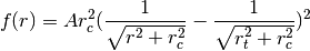
3D (deprojected) King model of the form:

Bases: pymodelfit.core.FunctionModel1DAuto
Moffat function given by:
Full Width at Half Maximum for this model - setting changes alpha for fixed beta
Bases: pymodelfit.core.FunctionModel1DAuto
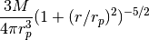
A Navarro, Frenk, and White 1996 profile – the canonical
 dark matter halo profile:
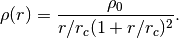
Where unspecified, units are r in kpc and rho in Msun pc^-3, although units can always be arbitrarily scaled by rescaling rho0.
Note
This form is equivalent to an AlphaBetaGammaModel with
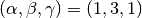 , but with a slightly
different overall normalization. This class also has a number of
helper methods.
, but with a slightly
different overall normalization. This class also has a number of
helper methods.
from Maller & Bullock ‘04 M_sun
Warning
These scalings are approximations.
| Parameters: | |
|---|---|
| Returns: | Virial mass in Msun |
from Maller & Bullock ‘04 M_sun
Warning
These scalings are approximations.
| Parameters: | |
|---|---|
| Returns: | Concentration parameter (rvir/rc) |
from Bullock ‘01 M_sun,kpc
Warning
These scalings are approximations.
| Parameters: | |
|---|---|
| Returns: | Virial radius in kpc |
Convert virial mass to vmax using the scalings here
Warning
These scalings are approximations.
| Parameters: | |
|---|---|
| Returns: | Maximum circular velocity in km/s |
from Bullock ‘01 km/s,M_sun
Warning
These scalings are approximations.
| Parameters: | |
|---|---|
| Returns: | Virial Velocity in km/s |
Computes virial velocity from virial radius and virial mass.
| Parameters: | |
|---|---|
| Returns: | Virial Velocity in km/s |
from Bullock ‘01 M_sun,kpc
Warning
These scalings are approximations.
| Parameters: | |
|---|---|
| Returns: | Virial mass in Msun |
Convert vmax to virial mass using the scalings here
Warning
These scalings are approximations.
| Parameters: | |
|---|---|
| Returns: | Virial mass in Msun |
Convert vmax to virial radius using the scalings here.
Warning
These scalings are approximations.
| Parameters: | |
|---|---|
| Returns: | Virial radius in kpc |
from Maller & Bullock ‘04 good from 80-1200 km/s in vvir
Warning
These scalings are approximations.
| Parameters: | |
|---|---|
| Returns: | Virial Velocity in km/s |
from Bullock ‘01 km/s,M_sun
Warning
These scalings are approximations.
| Parameters: | |
|---|---|
| Returns: | Virial mass in Msun |
Compute the Virial temperature for a given virial radius.
From Barkana & Loeb 2001:

 is the mean molecular weight, which is 0.59 for fully
ionized primordial gas, .61 for fully ionized hydrogen but singly
ionized helium, and 1.22 neutral.
is the mean molecular weight, which is 0.59 for fully
ionized primordial gas, .61 for fully ionized hydrogen but singly
ionized helium, and 1.22 neutral.  is the proton mass,
 is the Boltzmann constant, and
  is the virial
velocity.
is the virial
velocity.
| Parameters: | |
|---|---|
| Returns: | Virial Temperatur in Kelvin |
from Bullock ‘01 good from 80-1200 km/s in vvir
Warning
These scalings are approximations.
| Parameters: | Vvir (float) – Virial velocity in km/s |
|---|---|
| Returns: | Virial velocity in km/s |
Generates a new NFWModel with the given Mvir using the Cvir_to_Mvir() function to get the scaling.
Warning
These scalings are approximations.
| Parameters: | |
|---|---|
| Returns: | A NFWModel object with the provided Cvir and normalization set by the approximate scalings here. |
Generates a new NFWModel with the given Mvir using the Mvir_to_Cvir() function to get the scaling.
Warning
These scalings are approximations.
| Parameters: | |
|---|---|
| Returns: | A NFWModel object with the provided Mvir and concentration set by the approximate scalings here. |
Generates a new NFWModel with the given Mvir using the Mvir_to_Cvir and Rvir_to_Mvir() functions to get the scaling.
Warning
These scalings are approximations.
| Parameters: | |
|---|---|
| Returns: | A NFWModel object with the provided Rvir and concentration set by the approximate scalings here. |
Generates a new NFWModel with the given Vmax and R_Vmax.
| Parameters: |
|---|
See Bullock et al. 2001 for reflated reference.
| Returns: | A NFWModel object matching the supplied vmax and rvmax |
|---|
Returns the virial overdensity at a given redshift.
This method should be overridden if a particular definition of virial radius is desired. E.g. to use r200 instead of rvir, do:
nfwmodel.deltavir = lambda z:200
| Parameters: | z (scalar) – redshift at which to compute virial overdensity |
|---|---|
| Returns: | virial overdensity |
Returns the concentration of this profile(rvir/rc) for a given redshift.
Gets the mass within the virial radius (for a particular redshift)
Computes the mean density within the requested radius, i.e.
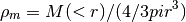
density in units of Msun pc^-3 assuming r in kpc
Get the virial radius at a given redshift, with deltavir choosing the type of virial radius - if ‘fromcosmology’ it will be computed from the cosmology, otherwise, it should be a multiple of the critical density
units in kpc for mass in Msun
Computes the circular velocity of the halo at a given radius. i.e.
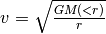 .
.
| Parameters: | r – The radius (or radii) at which to compute the circular velocity, in kpc. |
|---|
Additional keyword arguments are passed into integrateSpherical().
| Returns: | The circular velocity at r (if r is a scalar, this will return a scalar, otherwise an array) |
|---|
Computes the maximum circular velocity of this profile.
| Returns: | (vmax,rvmax) where vmax is the maximum circular velocity in km/s and rvmax is the radius at which the circular velocity is maximized. |
|---|
NFW Has an analytic form for the spherical integral - if the lower is not 0 or or if method is not None, this function will fall back to the numerical version.
Sets the model parameters to match a given concentration given virial radius and mass.
| Parameters: |
|
|---|
returns a new AlphaBetaGammaModel based on this model’s parameters.
Bases: pymodelfit.core.FunctionModel1DAuto
NFW Has an analytic form for the spherical integral - if the lower is not 0 or or if the keyword ‘numerical’ is True, this function will fall back to FunctionModel1D.integrateCircular
Bases: pymodelfit.core.FunctionModel1DAuto
Plummer model of the form
Bases: pymodelfit.core.FunctionModel2DScalarSeperable
A bulge modeled as a radially symmetric sersic profile (by default the sersic index is kept fixed - to remove this behavior, set the fixedpars attribute to None)
By default, the ‘n’ parameter does not vary when fitting.
Bases: pymodelfit.core.FunctionModel1DAuto
The Schechter Function, commonly used to fit the luminosity function of galaxies, in luminosity form:
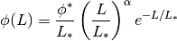
See also
SchechterMagModel, Schechter 1976, ApJ 203, 297
Compute Schechter derivative. if dx is not None, will fallback on the numerical version.
Analytically Compute Schechter integral using incomplete gamma functions. If method is not None, numerical integration will be used. The gamma functions break down for alpha<=-1, so numerical is used if that is the case.
Bases: pymodelfit.core.FunctionModel1DAuto
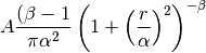
The Schechter Function, commonly used to fit the luminosity function of galaxies, in magnitude form:
![\Phi(M) = \phi^* \frac{2}{5} \ln(10) \left[10^{\frac{2}{5} (M_*-M)}\right]^{\alpha+1} e^{-10^{\frac{2}{5} (M_*-M)}}](../_images/math/c447091ca4b6153c7b8c4d62f4416d0e0ece0faf.png)
See also
SchechterLumModel, Schechter 1976, ApJ 203, 297
Compute Schechter derivative for magnitude form. if dx is not None, will fallback on the numerical version.
Analytically compute Schechter integral for magnitude form using incomplete gamma functions. If method is not None, numerical integration will be used. The gamma functions break down for alpha<=-1, so numerical is used if that is the case.
Bases: pymodelfit.core.FunctionModel1DAuto
Sersic surface brightness profile:
![A_e e^{-b_n[(R/R_e)^{1/n}-1]}](../_images/math/f686245842885c073b43ef3db2e90e205b0e8655.png)
Ae is the value at the effective radius re
Note
The Sersic profile is is mathematically identical to the Einasto profile (EinastoModel), although the parameterization is different. By Convention, Sersic generally refers to a 2D surface brightness/surface density profile, while Einasto is usually treated as a 3D density profile.
value at r=0
bn is used to get the half-light radius. If n is None, the current n parameter will be used
The form is a fit from MacArthur, Courteau, and Holtzman 2003 and is claimed to be good to ~O(10^-5)
Computes  exactly for the current sersic index, using
incomplete gamma functions.
exactly for the current sersic index, using
incomplete gamma functions.
Sets whether the exact Bn calculation is used, or the estimate (see getBn()).
| Parameters: | val – If None, nothing will be set, otherwise, if True, the exact Bn computation will be used, or if False, the estimate will be used. |
|---|---|
| Returns: | True if the exact computation is being used, False if the estimate. |
Computes for the current sersic index. If the
SersicModel.exactbn attribute is True, this is calculated using
incomplete gamma functions (bn_exact()), otherwise, it is
estimated based on MacArthur, Courteau, and Holtzman 2003
(bn_estimate()).
fit surface brightness using the SersicModel
r is the radial value,sb is surface brightness, zpt is the zero point of the magnitude scale, and kwargs go into fitdata
plots the surface brightness for this flux-based SersicModel. arguments are like fitDat