VNA Noise Analysis

This example records a series of sweeps from a vna to touchstone files, named in a chronological order. These are then used to characterize the noise of a vna

Touchstone File Retrieval

import mwavepy as mv
import os,datetime

nsweeps = 101 # number of sweeps to take
dir = datetime.datetime.now().date().__str__() # directory to save files in

myvna = mv.vna.HP8720() # HP8510 also available
os.mkdir(dir)
for k in range(nsweeps):
        print  k
        ntwk = myvna.s11
        date_string = datetime.datetime.now().__str__().replace(':','-')
        ntwk.write_touchstone(dir +'/'+ date_string)

myvna.close()

Noise Analysis

Calculates and plots various metrics of noise, given a directory of touchstones files, as would be created from the previous script

import mwavepy as mv
from pylab import *

dir = '2010-12-03' # directory of touchstone files
npoints = 3 # number of frequency points to calculate statistics for


# load all touchstones in directory into a dictionary, and sort keys
data = mv.load_all_touchstones(dir+'/')
keys=data.keys()
keys.sort()

# length of frequency vector of each network
f_len = data[keys[0]].frequency.npoints
# frequency vector indecies at which we will calculate the statistics
f_vector = [int(k) for k in linspace(0,f_len-1, npoints)]

#loop through the frequencies of interest and calculate statistics
for f in f_vector:
        # for legends
        f_scaled = data[keys[0]].frequency.f_scaled[f]
        f_unit = data[keys[0]].frequency.unit

        # z is 1d complex array of the s11 at the current frequency, it is
        # as long as the number of touchsone files
        z = array( [(data[keys[k]]).s[f,0,0] for k in range(len(keys))])
        phase_change = mv.complex_2_degree(z * 1/z[0])
        phase_change = phase_change - mean(phase_change)
        mag_change = mv.complex_2_magnitude(z-z[0])

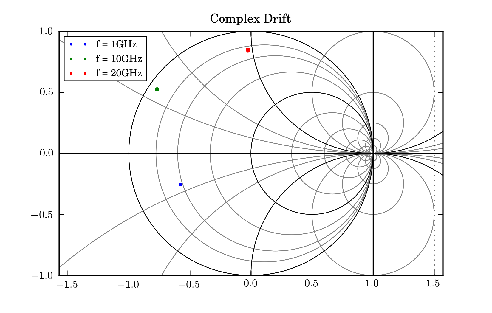
        figure(1)
        title('Complex Drift')
        plot(z.real,z.imag,'.',label='f = %i%s'% ( f_scaled,f_unit))
        axis('equal')
        legend()
        mv.smith()

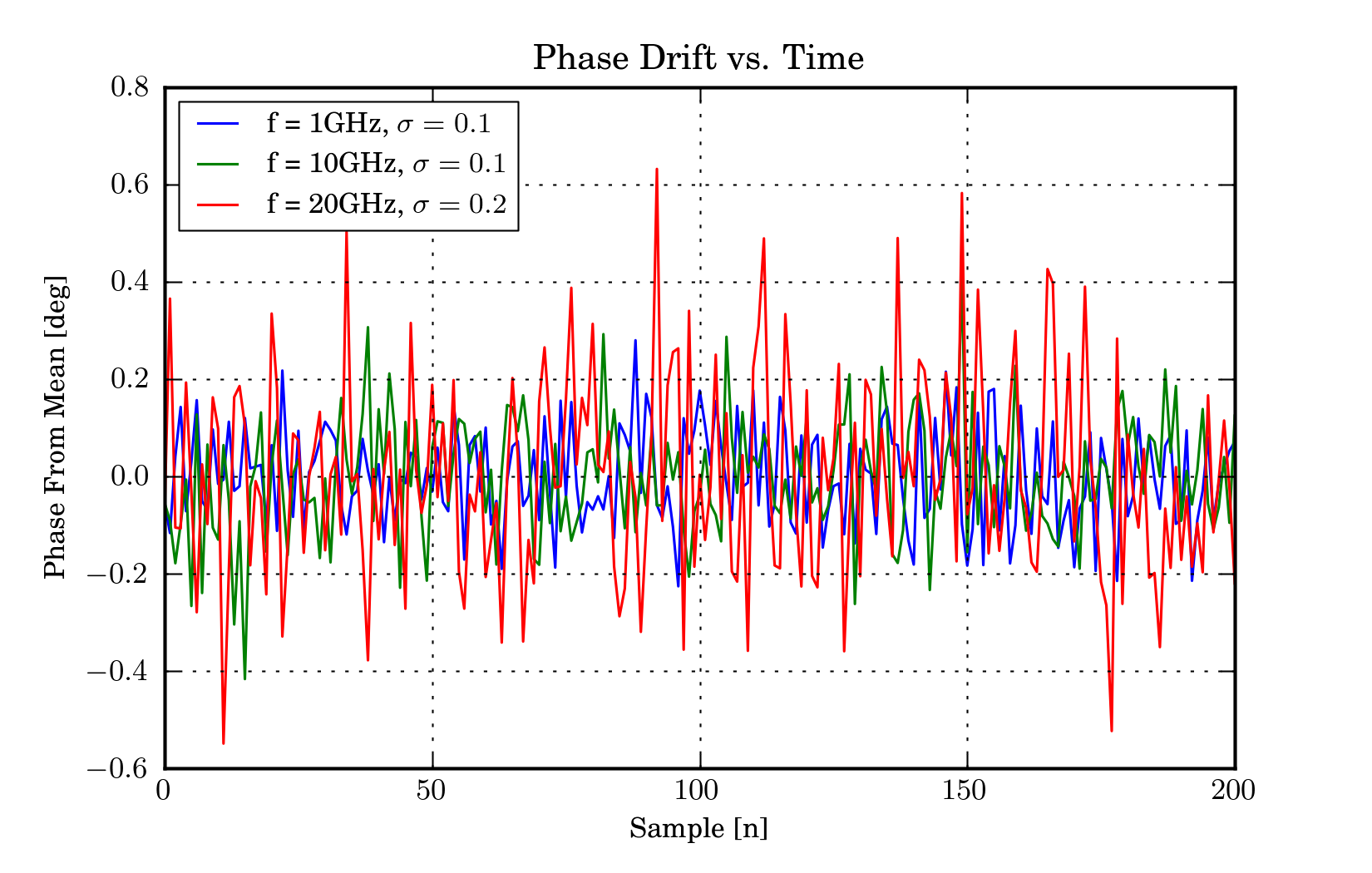
        figure(2)
        title('Phase Drift vs. Time')
        xlabel('Sample [n]')
        ylabel('Phase From Mean [deg]')
        plot(phase_change,label='f = %i%s, $\sigma=%.1f$'%(f_scaled,f_unit,std(phase_change)))
        legend()

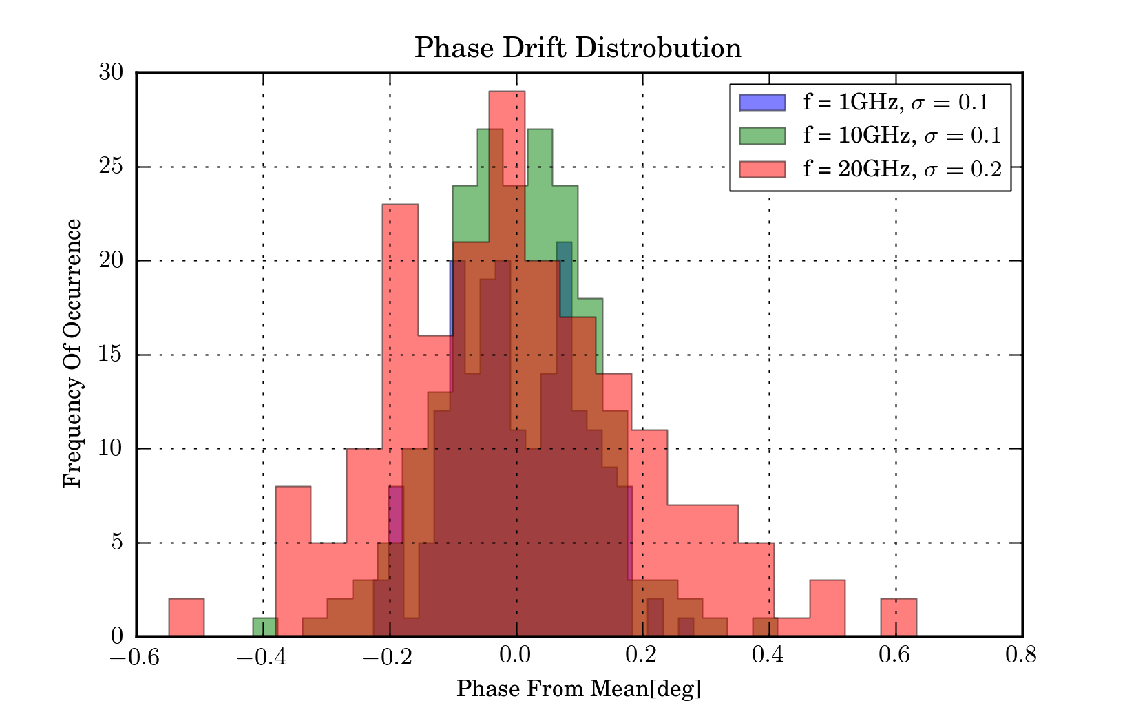
        figure(3)
        title('Phase Drift Distrobution')
        xlabel('Phase From Mean[deg]')
        ylabel('Frequency Of Occurrence')
        hist(phase_change,alpha=.5,bins=21,histtype='stepfilled',\
                label='f = %i%s, $\sigma=%.1f$'%(f_scaled,f_unit,std(phase_change)) )
        legend()
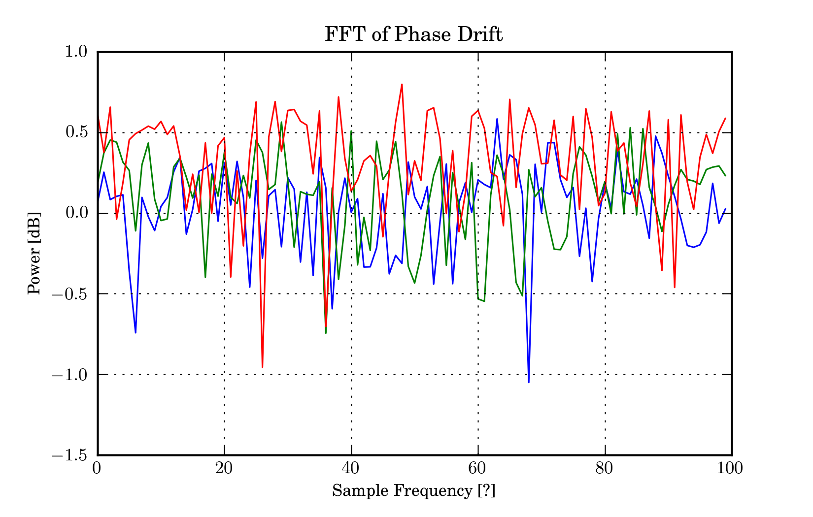
        figure(4)
        title('FFT of Phase Drift')
        ylabel('Power [dB]')
        xlabel('Sample Frequency [?]')
        plot(log10(abs(fftshift(fft(phase_change))))[len(keys)/2+1:])

draw();show();