Introduction
Contents
This is a brief introduction to mwavepy, aimed at those who are familiar with python. If you are unfamiliar with python, please see scipy’s Getting Started . All of the touchstone files used in these tutorials are provided along with this source code, and are located in the directory ../pyplots/ (relative to this file).
Creating Networks
For this turtorial, and the rest of the mwavpey documentation, we assume that mwavepy has been imported as mv. Whether or not you follow this convention in your own code is up to you:
>>> import mwavepy as mv
If this produces an error, please see Installation.
The most fundamental object in mwavepy is a n-port Network. Most commonly, a Network is constructed from data stored in a touchstone files, like so
>>> short = mv.Network('short.s1p')
>>> delay_short = mv.Network('delay_short.s1p')
The Network object will produce a short description if entered onto the command line:
>>> short
1-Port Network.  75-110 GHz.  201 points. z0=[ 50.]
Basic Network Properties
The basic attributes of a microwave Network are provided by the following properties :
- Network.s : Scattering Parameter matrix.
- Network.z0 : Characterisic Impedance matrix.
- Network.frequency : Frequency Object.
These properties are stored as complex numpy.ndarray’s. The Network class has numerous other properties and methods, which can found in the Network docs. If you are using Ipython, then these properties and methods can be ‘tabbed’ out on the command line. Amongst other things, the methods of the Network class provide convenient ways to plot components of the s-parameters, below is a short list of common plotting commands,
- Network.plot_s_db() : plot magnitude of s-parameters in log scale
- Network.plot_s_deg() : plot phase of s-parameters in degrees
- Network.plot_s_smith() : plot complex s-parameters on Smith Chart
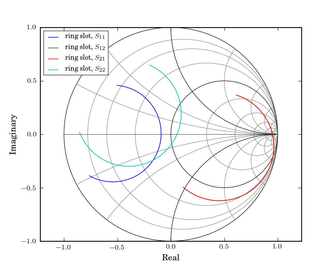
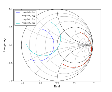
For example, to create a 2-port Network from a touchstone file, and then plot all s-parameters on the Smith Chart.
import pylab
import mwavepy as mv

# create a Network type from a touchstone file
ring_slot = mv.Network('ring slot.s2p')
ring_slot.plot_s_smith()
pylab.show()
(Source code, png, hires.png, pdf)
For more detailed information about plotting see Plotting.
Network Operators
Element-wise Operations
Element-wise mathematical operations on the scattering parameter matrices are accessible through overloaded operators:
>>> short + delay_short
>>> short - delay_short
>>> short / delay_short
>>> short * delay_short
All of these operations return Network types, so all methods and properties of a Network are available on the result. For example, the difference operation (‘-‘) can be used to calculate the complex distance between two networks
>>> difference = (short- delay_short)
Because this returns Network type, the distance is accessed through the Network.s property. The plotting methods of the Network type can also be used. So to plot the magnitude of the complex difference between the networks short and delay_short:
>>> (short - delay_short).plot_s_mag()
Another use of operators is calculating the phase difference using the division operator. This can be done
>>> (delay_short/short).plot_s_deg()
Cascading and Embeding Operations
Cascading and de-embeding 2-port Networks is done so frequently, that it can also be done though operators as well. The cascade function is called by the power operator, **, and the de-embedding operation is accomplished by cascading the inverse of a network, which is implemented by the property Network.inv. Given the following Networks:
>>> line = mv.Network('line.s2p')
>>> short = mv.Network('short.s1p')
To calculate a new network which is the cascaded connection of the two individual Networks line and short:
>>> delay_short = line ** short
or to de-embed the short from delay_short:
>>> short = line.inv ** delay_short
Connecting Multi-ports
mwavepy supports the connection of arbitrary ports of N-port networks. It accomplishes this using an algorithm call sub-network growth [1]. This algorithm, which is available through the function connect(), takes into account port impedances. Terminating one port of a ideal 3-way splitter can be done like so:
>>> tee = mv.Network('tee.s3p')
>>> delay_short = mv.Network('delay_short.s1p')
to connect port ‘1’ of the tee, to port 0 of the delay short:
>>> terminated_tee = mv.connect(tee,1,delay_short,0)
Sub-Networks
Frequently, the one-port s-parameters of a multiport network’s are of interest. These can be accessed by properties such as:
>>> port1_return = line.s11
>>> port1_insertion = line.s21
Convenience Functions
Frequently there is an entire directory of touchstone files that need to be analyzed. The function load_all_touchstones() is meant deal with this scenario. It takes a string representing the directory, and returns a dictionary type with keys equal to the touchstone filenames, and values equal to Network types:
>>> ntwk_dict = mv.load_all_touchstones('.')
{'delay_short': 1-Port Network.  75-110 GHz.  201 points. z0=[ 50.],
'line': 2-Port Network.  75-110 GHz.  201 points. z0=[ 50.  50.],
'ring slot': 2-Port Network.  75-110 GHz.  201 points. z0=[ 50.  50.],
'short': 1-Port Network.  75-110 GHz.  201 points. z0=[ 50.]}
References
| [1] | Compton, R.C.; , “Perspectives in microwave circuit analysis,” Circuits and Systems, 1989., Proceedings of the 32nd Midwest Symposium on , vol., no., pp.716-718 vol.2, 14-16 Aug 1989. URL: http://ieeexplore.ieee.org/stamp/stamp.jsp?tp=&arnumber=101955&isnumber=3167 |