Plotting

Contents

• Plotting
  • Magnitude
  • Phase
  • Smith Chart
  • Multiple S-parameters
  • Comparing with Simulation
  • Saving Plots

This tutorial illustrates how to create common plots associated with microwave networks. The plotting functions are implemented as methods of the Network class, which is provided by the mwavepy.network module. Below is a list of the some of the plotting functions of network s-parameters,

• Network.plot_s_re()
• Network.plot_s_im()
• Network.plot_s_mag()
• Network.plot_s_db()
• Network.plot_s_deg()
• Network.plot_s_deg_unwrapped()
• Network.plot_s_rad()
• Network.plot_s_rad_unwrapped()
• Network.plot_s_smith()
• Network.plot_s_complex()

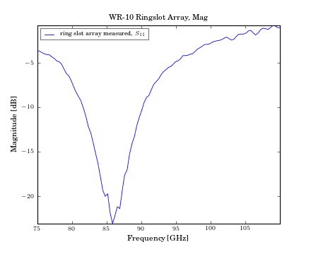
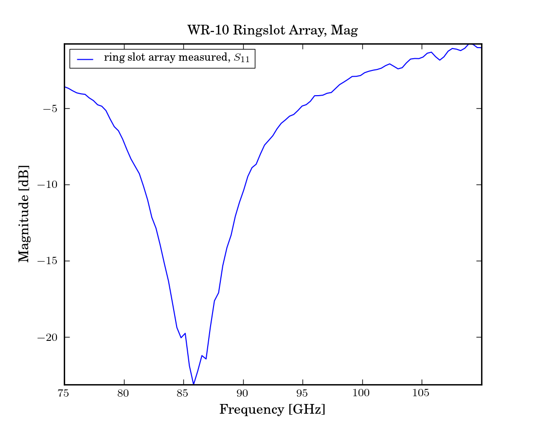
Magnitude

import pylab
import mwavepy as mv

# create a Network type from a touchstone file of a horn antenna
ring_slot= mv.Network('ring slot array measured.s1p')

# plot magnitude (in db) of S11
pylab.figure(1)
pylab.title('WR-10 Ringslot Array, Mag')
ring_slot.plot_s_db(m=0,n=0) # m,n are S-Matrix indecies
# show the plots
pylab.show()

(Source code, png, hires.png, pdf)

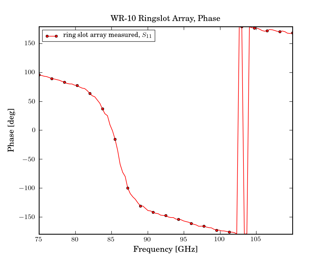
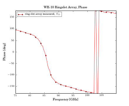
Phase

import pylab
import mwavepy as mv

ring_slot= mv.Network('ring slot array measured.s1p')
pylab.figure(1)
pylab.title('WR-10 Ringslot Array, Phase')
# kwargs given to plot commands are passed through to the pylab.plot
# command
ring_slot.plot_s_deg(m=0,n=0, color='r', markevery=5, marker='o')
pylab.show()

(Source code, png, hires.png, pdf)

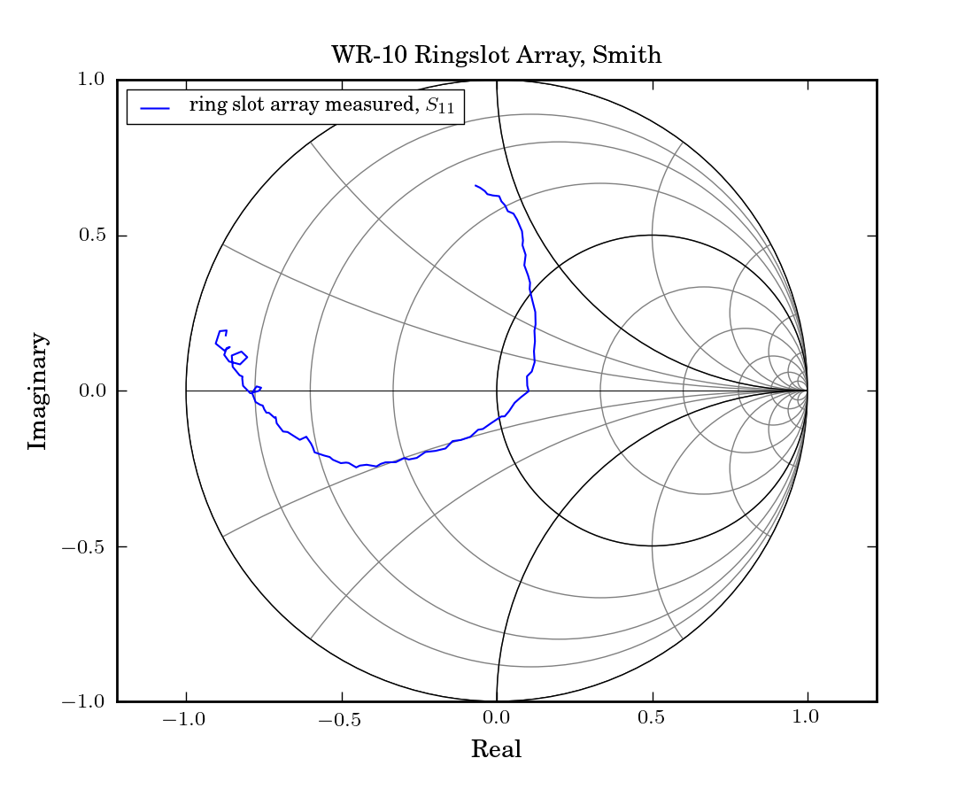
Smith Chart

import pylab
import mwavepy as mv

ring_slot= mv.Network('ring slot array measured.s1p')

pylab.figure(1)
pylab.title('WR-10 Ringslot Array, Smith')
ring_slot.plot_s_smith(m=0,n=0) # m,n are S-Matrix indecies
pylab.show()

(Source code, png, hires.png, pdf)

The Smith Chart can be also drawn independently of any Network object through the smith() function. This function also allows admittance contours can also be drawn.

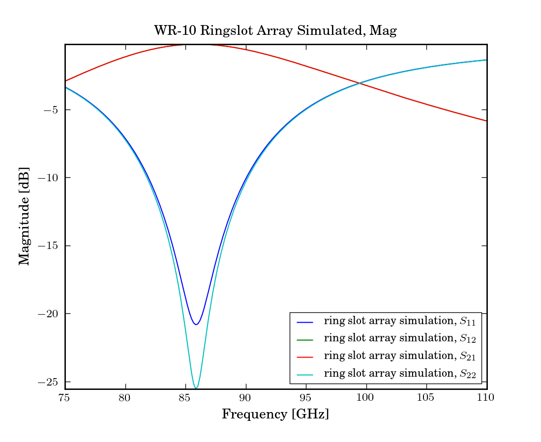
Multiple S-parameters

import pylab
import mwavepy as mv

# from the extension you know this is a 2-port network
ring_slot= mv.Network('ring slot array simulation.s2p')

pylab.figure(1)
pylab.title('WR-10 Ringslot Array Simulated, Mag')
# if no indecies are passed to the plot command it will plot all
# available s-parameters
ring_slot.plot_s_db()
pylab.show()

(Source code, png, hires.png, pdf)

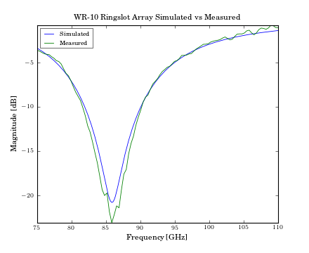
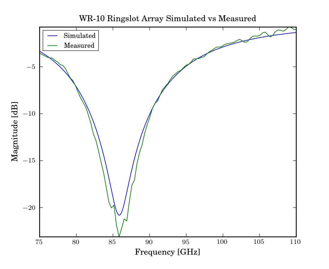
Comparing with Simulation

import pylab
import mwavepy as mv

# from the extension you know this is a 2-port network
ring_slot_sim = mv.Network('ring slot array simulation.s2p')
ring_slot_meas = mv.Network('ring slot array measured.s1p')

pylab.figure(1)
pylab.title('WR-10 Ringslot Array Simulated vs Measured')
# if no indecies are passed to the plot command it will plot all
# available s-parameters
ring_slot_sim.plot_s_db(0,0, label='Simulated')
ring_slot_meas.plot_s_db(0,0, label='Measured')
pylab.show()

(Source code, png, hires.png, pdf)

Saving Plots

Plots can be saved in various file formats using the GUI provided by the matplotlib. However, mwavepy provides a convenience function, called save_all_figs(), that allows all open figures to be saved to disk in multiple file formats, with filenames pulled from each figure’s title:

>>> mv.save_all_figs('.', format=['eps','pdf'])
./WR-10 Ringslot Array Simulated vs Measured.eps
./WR-10 Ringslot Array Simulated vs Measured.pdf